A while ago, I wrote about Meshtastic. At the time, Meshtastic was the thing everyone was talking about: tens of thousands of nodes sold, many products packaged by HELTEC, LILYGO, RAK, and Seeed Studio, and a large international community building a LoRa-based mesh network for long-range communication.

But Meshtastic was yesterday’s trend. Today, the new momentum is around MeshCore, with a significant part of the community migrating to it, especially because the required hardware platforms are largely the same. However, as we will see, MeshCore and Meshtastic are not the same thing. They are not really meant to replace each other, except perhaps for specific use cases where Meshtastic was not particularly well suited and where MeshCore provides more appropriate solutions.

This article introduces MeshCore from a technical and operational point of view, to help clarify what it is and how it works.

Why MeshCore ?

One of the interesting things about mesh networks is that there are dozens of different implementations, with architectures that can vary significantly depending on the problem they are trying to solve.

A typical example is Meshtastic. The original idea was to provide a way for people to communicate while hiking in the mountains, for instance, when they might need to contact others or call for help. In that context, the network relies on point-to-point communication between individuals to route messages across the group.

In other words, this is a network with no fixed infrastructure. The entire network is mobile, and the performance of LoRa makes it possible to cover long distances. From that initial concept came the idea of building a network capable of spanning large areas and, in the event of a disaster, allowing emergency messages to be sent.

This is an interesting and effective approach, but it also comes with limitations. Because there is no infrastructure to coordinate the network, messages are broadly propagated by the nodes. The protocol includes mechanisms to avoid excessive flooding, but the model remains bandwidth-intensive.

Of course, Meshtastic can use nodes that act as repeaters, but they work in essentially the same way as other nodes, with only a notion of priority. If you are hiking in the mountains, that concept of a repeater does not really make sense unless one has been installed at the top of a mountain ; that’s why it’s mainly a post design hack.

This type of problem is what Meshtastic was designed to address. It has also led many people to try to build large, fixed, terrestrial networks using the same solution. I have deployed a number of antennas myself with that goal in mind.

However, this system has limits in terms of deployment and scalability. Some of those limits are linked to the original requirement for very long-range coverage, which led to the use of high spreading factors and wide spectrum occupancy. This also makes its impact on other networks, its coexistence with technologies such as LoRaWAN, and its compliance with regulations less straightforward.

Meshcore comes with a different architecture, although it relies on a somewhat similar technological foundation: a mesh network. The main difference is that Meshcore separates devices into two types of profiles. The first is the repeater profile, which is part of the infrastructure and is generally expected, or even recommended, to be fixed. The second is made up of nodes that can send and receive messages.

This distinction changes the way the network behaves. In particular, it makes it possible to create routes for sending messages, instead of flooding messages in every direction without knowing where the recipient is located. This is an important gain when building a network intended to provide broad coverage, for example at the scale of a region or even a country.

This is one of the key differences between Meshcore and Meshtastic. Meshcore is more intended to be an out-of-band network with a long-term, durable infrastructure, on top of which nodes can transmit data. These nodes can send SMS-like messages, much like with Meshtastic, but they can also transmit telemetry.

Another important aspect is that Meshcore is not meant to rely on an Internet connection to relay messages between areas. The goal is to build a fully independent network. For that reason, it must be possible to administer infrastructure nodes remotely, and the protocol has been designed with this in mind.

As a result, the use cases are slightly different. Disaster coverage is still relevant, because these networks are lightweight to deploy, inexpensive, and can run on small solar panels. But overall, Meshcore is more oriented toward users such as radio amateurs who want to cover territory, optimize for long-distance performance, and build a large-scale, stable network.

This is the general difference in mindset between Meshcore and Meshtastic. In the next sections, we will look at how this translates from a technical point of view.

MeshCore, how it works ?

As mentioned earlier, in MeshCore we can simplify the model by saying that there are two main roles: the node role and the repeater role.

When deploying a device, the first question is therefore whether we want to deploy a node. A node is a device we can carry with us, connect to our smartphone, and use to send messages, for example saying hello on a public channel or sending a short message to a friend. It can also be used with a sensor that regularly sends information on its own.

This is one of the advantages of MeshCore: it makes it easy to build nodes whose purpose is not to send text messages, but rather to handle telemetry. In other words, MeshCore can also be used for IoT networks especially since it is based on an MIT license.

The other option is to deploy a repeater. In that case, the repeater should ideally be installed in a fixed position. Its location may be public or private, but it should, when possible, have a good antenna and be placed in a suitable location so that it can cover a wide area. Because this is a mesh network, the cost of the device and the repeater is the same. A device can be configured either as a node or as a repeater, which means a repeater only costs a few dozen euros to deploy.

You can find more details in my articles, for example on solar meshtastic. All the products presented here also work with MeshCore.

When it comes to creating a node on MeshCore, the team reused what worked well with Meshtastic: the ability to flash the device directly from the MeshCore web flasher. You simply select the type of product you have, and the rest is handled automatically. This makes the process accessible to almost everyone, which is one of the nice aspects of this ecosystem.

Configuration is done through the mobile application for regular nodes. For repeaters, it is usually done through the USB console, or, once the initial configuration has been completed, over the network by using your phone and a node to access the repeater.

There are plenty of resources explaining how to flash a node, set it up, and configure it. I encourage you to refer to those guides for the basics. Here, I will focus on different details instead.

End-user usage, like chat, is handled through a mobile application that is freely downloadable, although, to my knowledge, it is not open source. Some people criticize the fact that the app includes an in-app payment. In practice, this is a request to support the developer. It removes a limitation that requires users to wait 10 seconds before accessing the remote administration of a repeater. In my point of view, this is reasonable for two reasons.

• I was happy to contribute to the project, and this is a simple way to provide support, easier than an online payment that I probably would not have made.
• Remote configuration is rare enough that users who do not want to contribute can simply wait those 10 seconds without any real inconvenience.

My view, from a more industrial-oriented analysis, is that a mobile application is not a necessity for the protocol itself. Instead, in such context, we should favor direct access for configuration, either through a serial port or over the network, in order to make the overall operation more reliable.

MeshCore protocol 1-0-1

Overall, the principle is simple. When a node sends a message, it will usually switch to listening mode afterward to detect which repeaters retransmit it and to make sure the message has actually been repeated. If it has not, the node can trigger a retransmission. This makes it possible, when sending a message, to see how many repeaters received and repeated it. However, this number should not be interpreted as the total number of repeaters in the network. It only represents the repeaters that the node was able to detect within its own radio reception range.

As with Meshtastic, MeshCore uses a specific sync word. This makes it possible to filter LoRa traffic and avoid receiving messages from other systems. For example, MeshCore uses the sync word 0x12, while LoRaWan uses 0x34.This approach is becoming common practice, but it is not always a good one. As discussed in my blog post “Hidden side of LoRa“, the sync word is not just a byte that can be used for filtering. It is fundamentally a synchronization byte.

A message is sent from a node, and it can be sent in two different ways.

Flood mode (broadcast)

The first one is flood mode, or broadcast mode. In this case, no path is specified. The message is therefore repeated by every node that receives it. MeshCore can support up to 64 hops, although it is usually possible to configure shorter ranges. The message is itself sent as a flood, and the network propagates it broadly over repeaters.

ROUTE MODE

The second option is used when the sender wants to reach a specific recipient. This is one of the differences between MeshCore and Meshtastic. In this case, the sender can define the route to follow when sending the message. That route lists the identifiers of the repeaters that should be used to reach the destination.

This implies that the network topology is known, and that a stable route can be defined. Unlike other LoRa mesh networks, such as ORAMA-NET, the route is not dynamically computed by the network. It is static and defined by the sender.

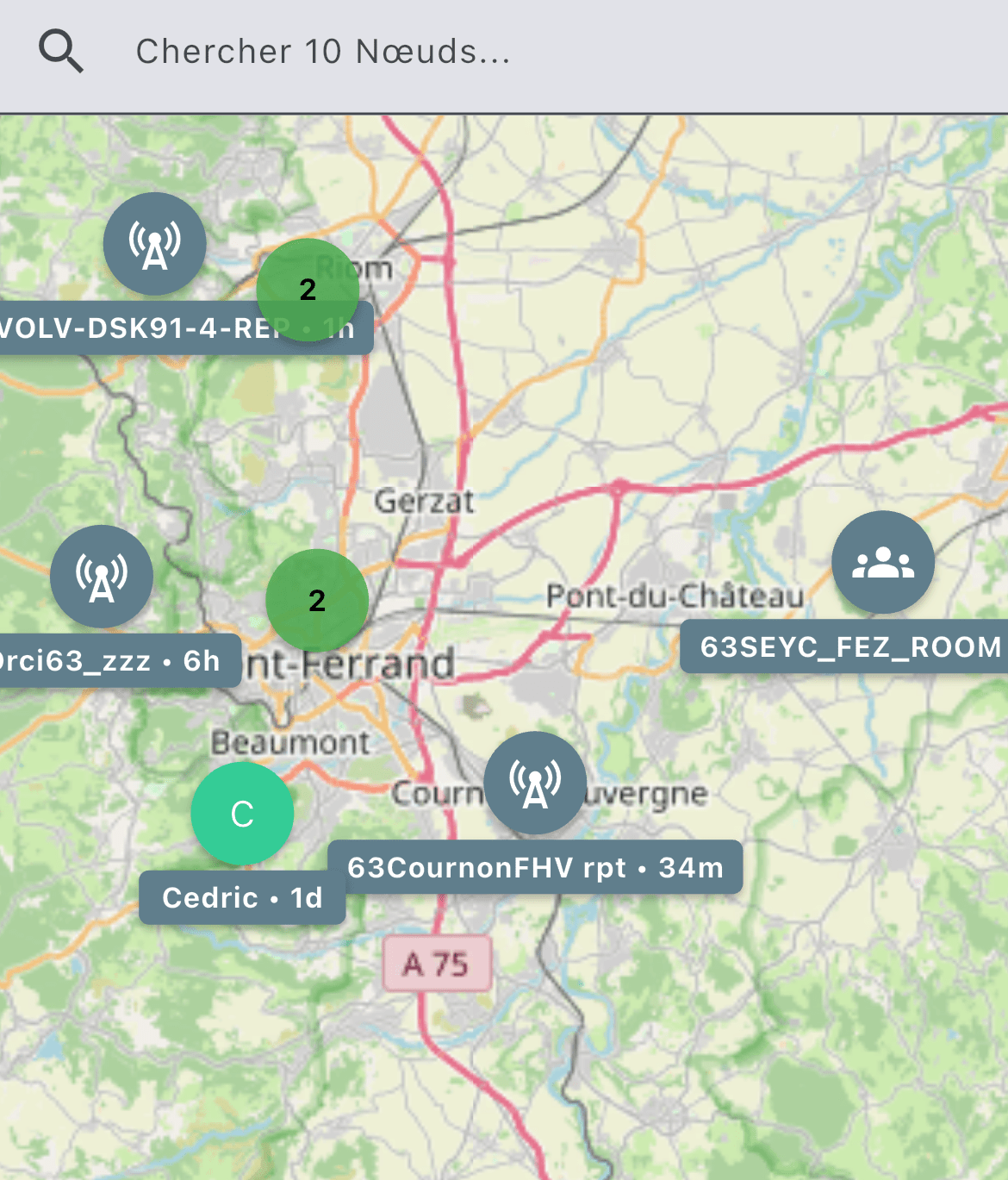
The network therefore needs to be reliable and stable enough for the route to keep working over time. It also requires network maps in order to find the necessary paths. To identify a path, each hop is defined by the identifier of the next repeater to reach.

We also need to build a map of the links between repeaters to ensure that the path is possible. But this can also be reconstructed from an initial flood message that arrived successfully, by reproducing the route taken by that last message.

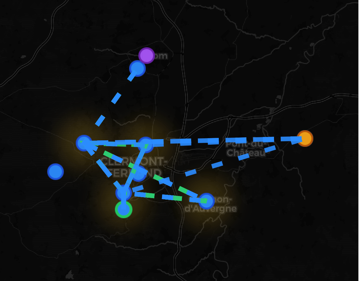
To keep frames at a reasonable size, the path is limited to 64 bytes. With 64 hops, this means that a single byte can be used to identify the next hop. In practice, this can create collisions within the same area, because this identifier is the first byte of the repeater’s public key.

Collisions can therefore happen, but in this context they are not necessarily a major issue. If two repeaters share the same identifier, both may retransmit the message, including one that was not originally intended to do so.

To reduce these collisions, the protocol was later extended to support addressing on 2 or 3 bytes. This significantly lowers the risk of collisions within a nearby network. However, this mode also comes with a constraint: it reduces the maximum number of hops, because the space reserved in the frame for the path is still limited to 64 bytes.

In practice, using 2-byte identifiers allows up to 32 hops, while using 3-byte identifiers allows up to 24 hops.

retransmitted or not ?

A repeater will always repeat a flood packet as long as it has not already done so. This is another difference with Meshtastic, which listens first and does not repeat a packet if it has already heard that someone else repeated it before. Here, the repeater will repeat every packet of type flood.

For packets that contain a path, the repeater will ignore the packet if it is not head of that path. If it is head of the path, it will take the packet and retransmit it.

Retransmission DELAY

When a repeater receives a frame to retransmit, there is no optimized spectrum management. Instead, the retransmission happens at a random point in time. In practice, this is a pure ALOHA-style access to the frequency band.

The time required to retransmit a frame depends on several parameters, some of which can be configured per repeater. Flood frames are handled differently from direct frames. For flood frames, the rxdelay parameter can be taken into account to potentially add a delay before the frame is processed based on the signal quality (score). This one is based on SNR, would not have been my choice. This is by default not activated.

rx_hold_ms = (rx_delay_base ^ (0.85 - score) - 1.0) × air_time_ms

Then, for all packets, some randomness is introduced into the retransmission timing. This is done through two mechanisms: a txdelay (flood) and direct.txdelay parameters, which allows the repeater to add a random delay delay based on the following elements. The estimate max duration is about 1200ms for default txdelay set to 0.5.

tx_jitter_ms = random int [0, 5 × air_time_ms × tx_delay]

The repeater mostly selects a random delay based on 50% of the estimated time on air of the transmission, generally multiplied by a random value between 0 and 5.

In other words, if the repeater density is high and they all use the same parameters, the probability that several repeaters choose a similar delay also becomes high. As a result, the risk of collision increases significantly. This type of network therefore requires repeaters to be relatively far apart from each other, and high repeater density in the same area should be avoided.

This part is rather complex. I would even say it may be a little too complex for the intended goal. However, it is fairly well documented in the following link.

Retransmission and path

There is also an important and particularly interesting mechanism for determining paths. When a flood packet is sent in this case, and as long as the path is not empty, each repeater adds its own ID, using 1, 2, or 3 bytes, inside the path. This allows each receiver to know which path was used to reach it. A flood-type message will increase in size as it is repeated across the network.

In contrast, a direct message with a predefined path will gradually decrease in size. Each repeater that recognizes itself in the path removes itself from the route list before retransmitting the message, placing the next required hop at the beginning of the message. As a result, the path becomes shorter step by step.

A sender can know the path taken by its message by receiving a return path message content type, which allows this information to be sent back to the sender to build a direct route in a later message.

Packet vs PAYLOAD

MeshCore uses two clearly distinct concepts: the packet and the payload.

The packet can be seen as the layer 3 component. It defines the rules for message transmission and routing. As discussed earlier, this layer may be modified during transmission, which means it cannot be encrypted. Instead, it is protected through mechanisms such as LoRa frame CRC, whose role is to validate that the frame has been received correctly.

The payload, on the other hand, is the message encapsulated inside the packet and belongs to the application layer. MeshCore includes several predefined application-level functions, such as sending messages or, as mentioned previously, acknowledging a message by returning the route that was used to receive it. There are other functions as well, but I will not cover them here.

This payload is encrypted end to end and can be encrypted in different ways depending on the type of communication. For a direct message, encryption relies on the keys of the sender and the recipient. For public communication spaces, it uses keys known by all participants. For private group communication, it relies on shared group keys.

I will not go into the security aspects in detail. I have read a long blog post on this topic, and overall the design appears to be serious. From a protocol perspective, I have not identified any specific issue, especially since the protocol does not manipulate the payload itself. The payload is handled only at the application level, typically by the companion applications being used. At the packet level, there is no mechanism in place, not even to authenticate the packet sender. Security is entirely delegated to the payload layer, which can introduce both limitations and risks, depending on the payload type. As a result, the security level may not be consistent across payloads. On the other hand, this approach makes it possible to implement a specific security model within a custom payload if needed. I do not see this as a drawback, because it makes it possible to adapt the level of security to the value of the data being transmitted without impacting the entire protocol.

However, direct communication between two people requires sharing public keys in advance so they can communicate with each other. This public key exchange is usually done through a QR code or a link that must be added to the application before the exchange can take place.

This blog post from Alainx277 is also an interesting reading because it takes a rather critical look at security from several angles. The first point concerns the codebase, which I hope has evolved since the article was written. It also discusses how security is handled at the payload authentication level, although the author’s assumption that a message is required every five seconds seems poorly aligned with the reality of this type of network.

MeshCore radio setup

The radio configuration can be modified by the user and should be adapted to the region where the device is deployed. In this section, we will review the parameters used for the European region, explain what they mean, and describe their impact on communications.

Frequency, bandwidth, power and duty-cycle

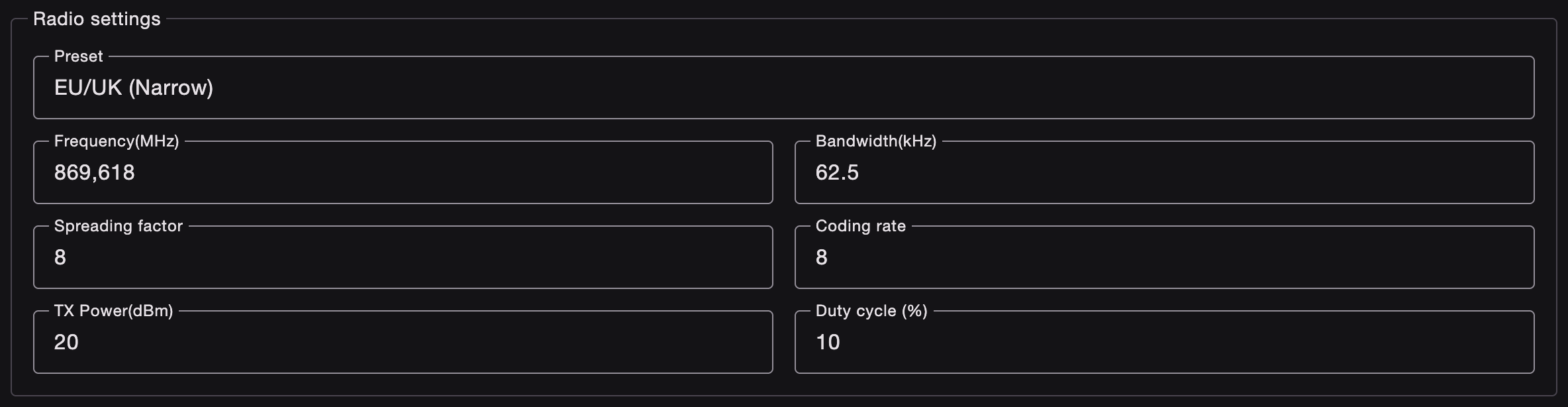
For Europe, we generally use the EU/UK preset in Narrow, which defines the use of a narrowband configuration. With this setting, we use a frequency of 869.618 MHz and a bandwidth of 62.5 kHz. This means that the band being used is at the upper end of the 869 MHz band, which extends up to 869.650 MHz. This allows us to use a 10% duty cycle and a transmit power of up to 500 mW.

This has several advantages. Typically, LoRaWan uses a 125 kHz bandwidth, and using a narrower bandwidth helps avoid collisions with LoRaWAN traffic on this important frequency band, since it is the band used for downlinks.

By operating at 869.618 MHz, we are very close to the edge of that band. In my point of view, to avoid rejection issues on adjacent bands, it would have been preferable to shift the center frequency slightly closer to the middle of the band.

The power can therefore be increased up to 27 dBm. This will depend on the node’s ability to transmit at that level. In practice, nodes are often based on chips typically used in end devices, which means their transmission power is usually limited to 20 dBm or 22 dBm, and rarely goes beyond that.

Pay attention to the duty cycle, since the default value is 50%, while the regulation for this frequency band only allows a 10% duty cycle. This is therefore a parameter that must be adjusted during configuration.

spreading factor & coding rate

A spreading factor of 8 determines the rate at which bits are transmitted and the number of bits sent with each chirp. In LoRa, SF8 is considered a relatively fast spreading factor. It therefore provides a higher data rate, but the trade-off is reduced radio performance in terms of range. The maximum achievable sensitivity is around -136 dBm, which makes it a reasonable option for covering long distances. Using a relatively narrow bandwidth reduces the data rate, but improves sensitivity in this case.

A coding rate of 8 means that for every 4 useful bits sent, 8 bits are transmitted, resulting in a redundancy factor of 2. This makes it possible to lose some data, or to have collisions on some chirps, without necessarily losing the entire frame, as long as enough information remains to reconstruct the transmission. In other words, it increases the likelihood that a message is correctly delivered to its recipient.

The theoretical throughput in terms of useful transmitted data is around 975 bits per second, which is generally fast for Long Range IoT transmissions. For short frames, the impact of overhead, headers, and related processing reduces the effective throughput. In practice, it is more realistic to consider data rates around 500 to 600 bits per second.

Advertising parameters

Each node sends advertising information to introduce itself to the network and indicate whether it is still active. These advertisements are sent in several ways.

The first type is zero-hop advertising. It is sent only to nearby neighbors, so it is not relayed through the network. This corresponds to the advert_interval parameter, which is set here to 240 minutes, or 4 hours.

The second type is sent in flood mode, meaning it is propagated through the network. In this case, it is sent less frequently, with an interval expressed in hours. Here, the interval is 24 hours, or one day. This flood advertisement is not sent across the entire network: it is limited by the number of hops, set here to 8. This is controlled by the flood_max parameter.

These parameters should be adjusted based on the size of the network and the number of devices it contains, in order to avoid saturating it. Advertisement parameters are used by both repeaters and nodes, allowing them to report their current state.

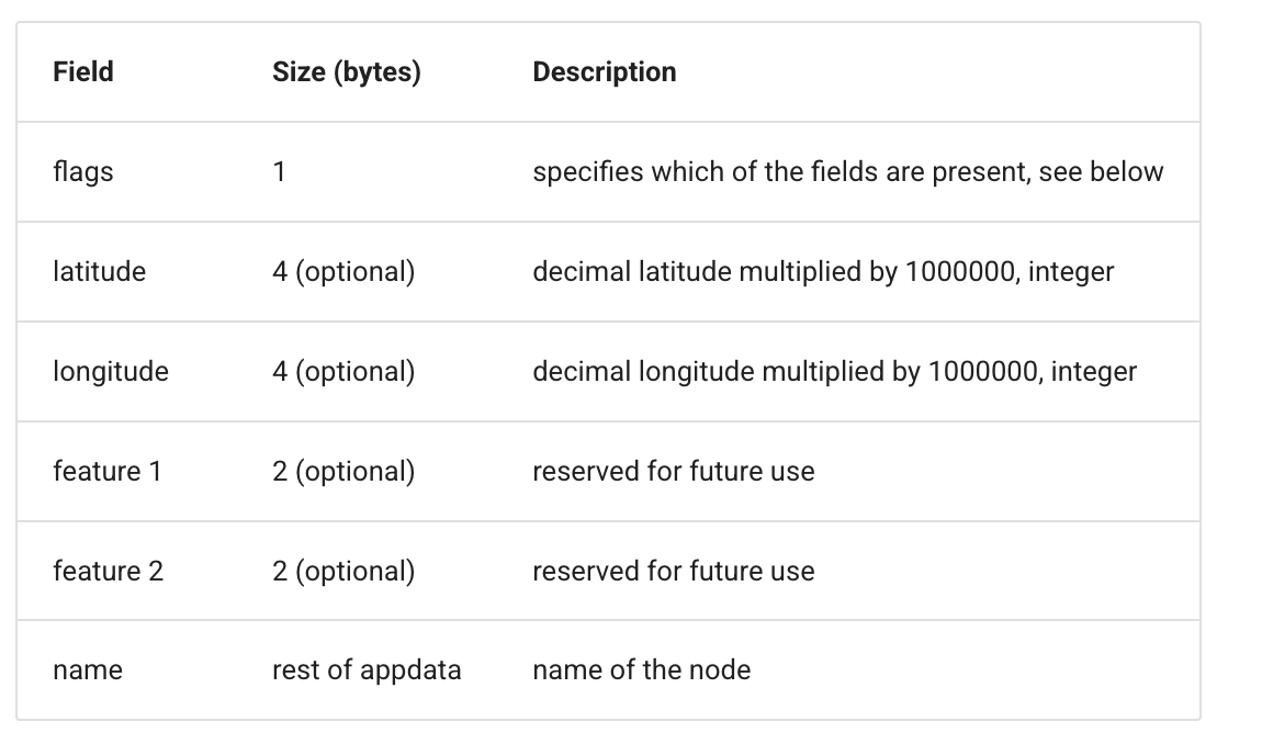
An advertisement contains several pieces of information, including telemetry data. It can also include a GPS position, making it possible to locate the different devices.

Advanced settings

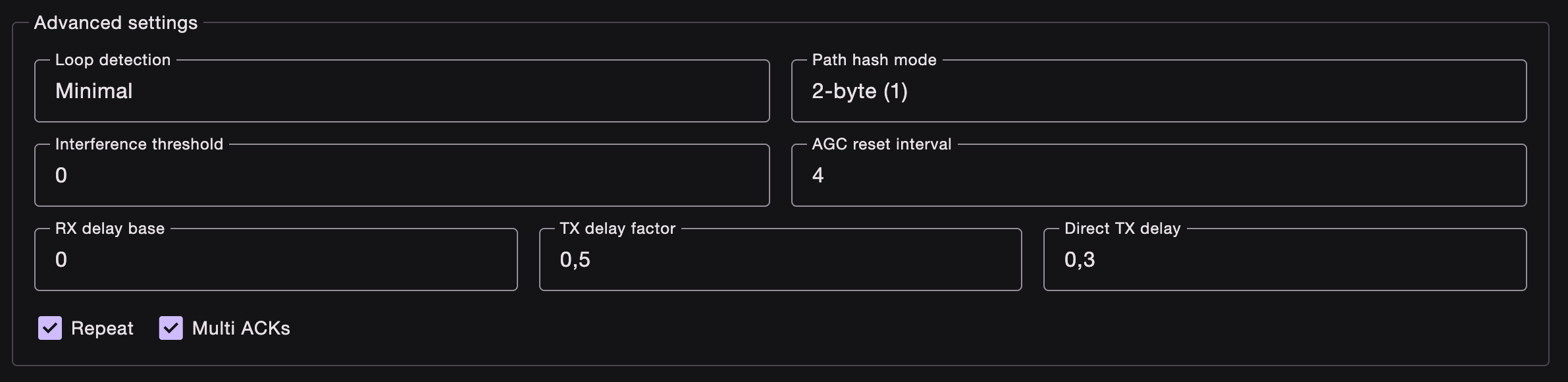
Loop detection prevents a packet from being forwarded if the same repeater identifier appears multiple times in the path. The issue, as discussed earlier, is that this identifier is not unique, so collisions can occur. Different strategies can therefore be used depending on the network and the expected level of risk.

Loop detection can be disabled, but this introduces the risk that frames may circulate endlessly (up to max hop). It can also be configured in a minimal mode. In that case, the system checks that the identifier does not appear more than four times for routes using one-byte packets, or more than twice for routes using two-byte packets, for example. Other modes are also possible, such as strict mode. In strict mode, all frames are dropped as soon as the hash of the ID is already present in the path. This can become a problem in networks where identifier collisions are expected.

The path mode defines how many bytes are used for the route identifier, which is used to identify each repeater that defines the route. With a value of 1 byte (mode 0), only the first byte of the public key is used to identify the repeater. With only 255 possible values, the risk of collision becomes significant. This connects back to the previous point about loop detection.

For networks that are expected to become large, for example at a country scale, it may be preferable to use a 2-byte identifier. This also means that the maximum path length is reduced, since the maximum space available to store the route is 64 bytes. With 2-byte identifiers, a defined route can contain up to 32 hops. Overall, this is a good compromise.

The last mode uses 3 bytes and is intended for very large networks, or for cases where the goal is to minimize the risk of identifier collisions as much as possible.

It is worth noting that this parameter was introduced in later versions of the protocol. As a result, some repeaters running older firmware only support paths using 1-byte identifiers.

The AGC reset interval parameter is slightly trickier. It resets the automatic gain control system on the receive path. In practice, the device updates its receive amplifier based on the surrounding noise level. If there is very little noise around the receiver, it can increase its gain to receive signals with higher sensitivity. Conversely, if the noise level is high, it will reduce the gain instead. This is a dynamic configuration of the receive gain. In this case, it is updated every 4 seconds when the parameter is set to 4. The system can be disabled by setting the value to 0.

The three fields, RX delay base, TX delay factor, and TX direct delay, are the parameters discussed earlier. They are taken into account when a frame is received to determine when it should be retransmitted. These parameters are not expressed in units such as milliseconds or any other direct time value. They are factors applied based on other parameters and on the frame’s transmission time.

RX delay base only applies to flood packets. In general, when its value is greater than 1, packets with a low SNR, (signal-to-noise), are delayed for longer, while packets with a high SNR are prioritized. When the value is between 0 and 1, the logic is reversed: frames with a low signal-to-noise ratio are prioritized instead. The usual configuration is to set it to 0, which disables this feature. In all cases, the packet will be retransmitted. The purpose of this feature could be, for example, to limit the risk of collisions by postponing certain transmissions, since, as mentioned earlier, the temporal diversity of retransmissions is not very high.

The TX delay factor also applies to flood-type frames. This factor is multiplied by the time the frame took to be transmitted, which roughly amplifies the effect of the random timing calculation that selects a value between 0 and 5. As a result, it slows down transmission by spreading out retransmissions over time. However, if the TX delay factor is the same across all nodes, it will not reduce the risk of collisions. The value becomes more useful within a network when different TX delay factors are used, so that even if multiple nodes draw the same random number, their retransmissions do not happen at exactly the same time. For this reason, it is more of a parameter that should be left to each repeater’s discretion rather than configured globally for an entire network.

The direct TX delay works in exactly the same way, except that it applies to messages that are not flood-type messages. By default, its value is lower, which does not change much overall, except that the message can be delivered faster. In that case, the collision risk remains the same.

Since the transmission time of a reasonably average-sized frame is around 250 milliseconds, each unit of the tx delay parameters will influence the frame transmission time by roughly that order of magnitude. With the default value of 0.5 for flood, we can expect wait times of around 125 milliseconds, applied between 0 and 5 times depending on the value drawn. In practice, this means a maximum delay of roughly 625ms when for direct message it’s more about 200ms with default value 0.3.

These considerations are also interesting because the path that could be automatically established for a direct message may be based on a message that was previously transmitted by flood. Its arrival time will depend on these random values and parameters. As a result, the first message received is not necessarily the one that followed the best path. It is simply the one that arrived the fastest, and this may need to be taken into account when calculating a route. I do not know exactly how the algorithm works internally, but if the route is chosen manually, I think these factors should be considered. They require continuous mapping to visualize what is happening and to avoid pushing everyone toward minimum tx delay values, since these values can drastically reduce collisions.

The multi-hack parameter simply consists of sending two acknoledgement frames instead of a single ack frame. This is a good recommendation because natural frame loss is significant on radio network (like 15%). Sending the frame twice, combined with a 4/8 coding rate, adds enough information redundancy to achieve a very good reception rate (like 99%).

Region filtering

To prevent flooded messages from reaching destinations that are too far away and unnecessarily saturating the network, it is possible to define the notion of a region. These regions can also be hierarchical. For example, we could imagine a structure based on a country, then a region, then a city. With this approach, a broadcast message could be limited to a specific city instead of being propagated across the entire network.

For this to work, the zones need to be consistently defined across the network. Since they are not standardized and are represented as character strings, all participants in the network must agree on the naming and structure of these zones. This ensures that a message sent to a given zone can be correctly identified and filtered.

By default, if no zone is defined, the filtering settings accept all packets. However, if a zone is defined, for example “France”, then a packet presented as coming from another zone will not be repeated by relays configured to filter only the “France” zone. The protocol does not carry string values related to the zone. Instead, it carries a 16-bit hash value, which acts as a transport code and is used to check whether there is a match.

Meshcore frame

A MeshCore frame therefore has the following format, which is fairly simple. There is no overhead in this frame: the information required at the application level is only carried in the payload. Depending on the service, this payload can contain more or less detailed information.

This structure is well designed compared to Meshtastic, which tends to create very long frames with many redundant or unnecessary fields. Here, the frame contains only what is needed to fulfill its purpose, while higher-level services can be built on top of it. The network layers are also fairly well respected.

Conclusion

It is difficult to write a real conclusion here, except to say that MeshCore is a particularly interesting mesh protocol. Its popularity comes largely from user-oriented applications, especially local out-of-band messaging. This makes it a compelling way to introduce people to these technologies at a low cost and in a playful, accessible way.

That said, I think the technology also has real value for industrial use cases, especially in sectors where mesh networking brings concrete benefits. The first one is infrastructure cost: a repeater only costs a few dozen euros. More importantly, it is possible to build a fully autonomous, solar-powered system at a very reasonable cost (~50€) compared with a LoRaWAN-type infrastructure, while also avoiding the need for an internet connection.

MeshCore is therefore an interesting protocol: easy to implement in connected devices, easy to extend, and built on a solid foundation. It is also possible to define custom payloads if the existing ones do not fully match more industrial requirements.

Overall, this is a topic I will probably explore further. The main limitation today is perhaps the lack of deeper technical documentation. I spent quite a lot of time writing this article and had to look for information in several places, including the source code, to really understand how things work. This is something that could improve over time, especially if a more industrial ecosystem starts to develop around the protocol.